
The previous post introduced the topic of phase transitions and how they might be used as models for earthquakes and markets. Phase transitions occur in a wide variety of physical, social, and engineered systems when nonlinear processes are present. In those contexts, they are also called regime changes or tipping points. This post will discuss some of the technical details of the theory of phase transitions and how these relate to the stability of earthquake fault systems and markets.
For purposes of illustration, let us assume that there exists a function U[ϕ] that describes the “cost” associated with creating a given state ϕ of a system. In physics, such a function is called a free energy function. In biology, the function -U[ϕ] is usually termed a fitness function. For markets, -U[ϕ] can be considered to be a utility function in the sense of Bernoulli.
In physics, the variable ϕ is called an order parameter because it is associated with the evolution of the system from one state of order to another. The evolution may proceed suddenly or perhaps via a series of random, chaotic, or intermediate states.
In physics, systems evolve to minimize the free energy or the cost. In biology, systems evolve towards maximum fitness. Likewise, we can consider that markets evolve to maximize utility. These considerations provide a context for the dynamics of these systems, and a rationale for their evolution in time.
To be more specific, let’s look at an example. Let’s define a cost function:
U[ϕ] = -fϕ + ϵϕ^2 + αϕ^4
Here, the function U[ϕ] describes the free energy or cost required to create the system state ϕ. In physics, this function is identified with the Landau Theory of phase transitions.
Let’s further assume that α is a positive number, while f and ϵ can be either positive or negative. A plot of this function in four specific cases can be seen below.
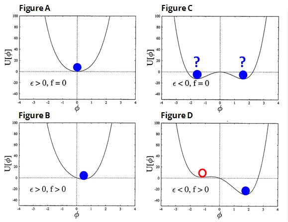
In figure A, there is only one minimum in the center at ϕ=0. The principle of minimum cost (minimum free energy) means that the system remains at the stable state ϕ=0 indicated by the blue dot. This is the only equilibrium state.
In figure B, the minimum state has been shifted to the right as f is increased, so the equilibrium state ϕ has a positive nonzero value. This is an example of an equilibrium transition, since in going from a to b, a continuous change in variable f is associated with a stable, reversible, continuous change in state ϕ. There is still just one equilibrium state.
In figure C, there are now two minima (two stable states) and the system could be in either of them. There are two possible equilibrium states, and the choice of which to occupy is determined by the details of evolution of the system. A selection rule of some sort would be needed to determine which state the system occupies.
Figure D shows the most interesting example. Now there are two minima, one of which is a local minimum (left hand state, red circle), and the other of which is the global minimum (right hand state, blue dot).
In accord with the principle of least cost or minimum energy, the system state would normally correspond to the right hand state (blue dot). However, it is possible to imagine dynamical processes that lead to the system residing in the left hand, local minimum state (red circle). An example of such a process for a driven earthquake model has been described here.
States of metastable equilibrium can often be long-lived, a condition that John Maynard Keynes essentially described by the pithy statement that “the market can stay irrational longer than you can stay solvent”. Phenomena associated with this state of metastability also include hysteresis.
After some average period of time termed the metastable lifetime, the state of the system will transition suddenly and spontaneously from the left hand, higher energy state, to the right hand, lower energy state. This spontaneous transition in state is the model for an earthquake or market crash.
Conditions leading to the decay from metastablity are associated with tipping points. Here it is said that the system has nucleated to the state of lower energy. These nucleation events are the first order phase transitions described in the previous post.
Relating these abstract ideas to the dynamics of earthquakes and markets and the stability of these systems is a subject that we will take up in a future post.
John Rundle is a Distinguished Professor of Physics and Geology at the University of California, Davis. We had the pleasure of meeting Professor Rundle through the Santa Fe Institute and were intrigued by his work on the dynamics of complex systems, specifically in the geosciences. His work on earthquake and hazard forecasting, and the similarities of these hazards to the financial markets expanded how we think about market movements and crashes.
Read his first post: Using Earthquakes to Understand Markets: Why and How
Read his third post: Earthquakes and Markets: Hysteresis